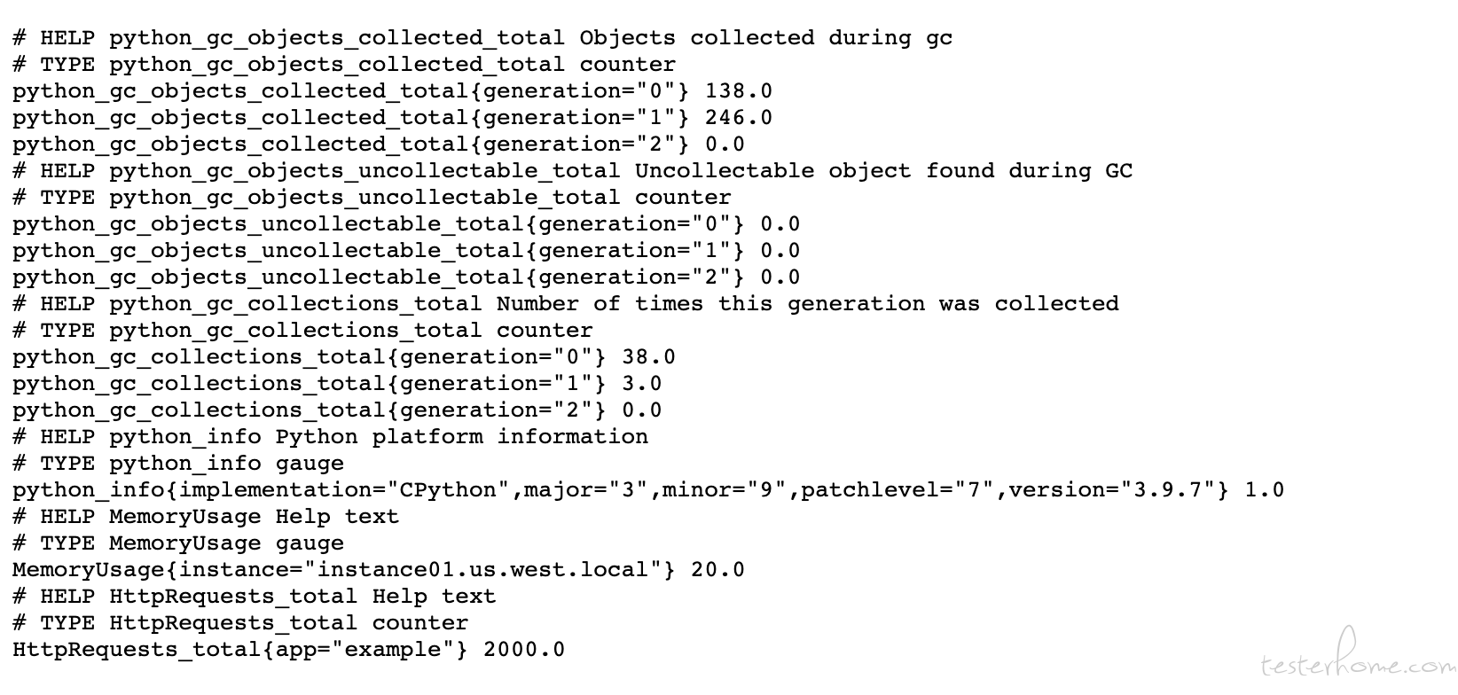
之前讲过普罗米修斯自己就是一个时序数据库, 它从 exporter 拉取的数据都会按时间戳保存到对应的文件里,这个时序数据库默认会保存 14 天的数据。 而它自己也开发了一套名为 PromQL 的类 SQL 的查询语言用来从各种维度让用户来查询并计算监控的数据。 我们先来看一下我自己编写的 exporter 的接口, 看看它向普罗米修斯的主服务返回的监控数据是什么样的。
其中 # 开头的是某个或者某些指标的帮助文档, 而非 # 开头的每一行表示当前 Exporter 采集到的一个监控样本。由于我是使用普罗米修斯的 python client 编写的 exporter, 所以它自带了 python 的多个监控指标。 而下面的MemoryUsage 和HttpRequests 就是我自己定义的监控指标了。 这其中MemoryUsage 和HttpRequests 是指标名称, 花括号内的是这个指标的 label, label 是个非常重要的机制, 它把相同的监控指标按自定义的 label 类型进行分类,比如这个监控数据是哪个机器的, 哪个机房的等等。 是编写 exporter 的人定义上去的, 目的是在后续使用 PromQL 的时候用户可以用 label 把监控数据进行分类查询 。 比如用户想要抓取每台机器上的 CPU Load 数据,分别显示出来 。 那它就要在查询 cpu_load15 的时候用 label 进行分组了。 最后面的浮点数值就是监控数据的值了。
^
 │   . . . . . . . . . . . . . . . . .   . .   node_cpu{cpu="cpu1",mode="idle"}
 │     . . . . . . . . . . . . . . . . . . .   node_cpu{cpu="cpu1",mode="system"}
 │     . . . . . . . . . . . . . . . .   . .
 v
   <------------------ 时间 ---------------->
在时间序列中的每一个点称为一个样本(sample),样本由以下三部分组成:
如下图:
<--------------- metric ---------------------><-timestamp -><-value->
http_request_total{status="200", method="GET"}@1434417560938 => 94355
http_request_total{status="200", method="GET"}@1434417561287 => 94334

http_request_total{status="404", method="GET"}@1434417560938 => 38473
http_request_total{status="404", method="GET"}@1434417561287 => 38544

http_request_total{status="200", method="POST"}@1434417560938 => 4748
http_request_total{status="200", method="POST"}@1434417561287 => 4785
在普罗米修斯中,有 4 种类型的指标:Counter, Gauge, Histogram 和 Summary
counter 类型的指标是一个只增不减的计数器, 我们上面的 http_request_total 还有 cpu 相关的信息都是属于 counter 类型的。 一般在定义 Counter 类型指标的名称时推荐使用_total 作为后缀。 一般 counter 类型的指标都会配合内置函数 rate 或者 irate 来完成指标的计算。比如我想统计某台机器上监控的进程 CPU 的使用率,那么可以使用这条语句查询:
rate(process_cpu_seconds_total{kubernetes_io_hostname="xxxxxxxx"}[5m])
这里解释一下这个查询的含义。这里主要解释 3 个地方
与 Counter 不同,Gauge 类型的指标侧重于反应系统的当前状态。这类指标的样本数据可增可减。常见指标如:node_memory_MemFree(主机当前空闲的内存大小)、node_memory_MemAvailable(可用内存大小)都是 Gauge 类型的监控指标。通过 Gauge 指标,用户可以直接查看系统的当前状态。
Histogram 和 Summary 我用的不多,所以还是用网络上一个例子来说吧, 他们主要用于统计和分析样本的分布情况。 他们类似在性能测试中我们喜欢查看 TP 99, TP 95, TP 90 这样的指标。Histogram 和 Summary 都是为了能够解决这样问题的存在,通过 Histogram 和 Summary 类型的监控指标,我们可以快速了解监控样本的分布情况。
例如,指标 prometheus_tsdb_wal_fsync_duration_seconds 的指标类型为 Summary。 它记录了 Prometheus Server 中 wal_fsync 处理的处理时间,通过访问 Prometheus Server 的/metrics 地址,可以获取到以下监控样本数据:
# HELP prometheus_tsdb_wal_fsync_duration_seconds Duration of WAL fsync.
# TYPE prometheus_tsdb_wal_fsync_duration_seconds summary
prometheus_tsdb_wal_fsync_duration_seconds{quantile="0.5"} 0.012352463
prometheus_tsdb_wal_fsync_duration_seconds{quantile="0.9"} 0.014458005
prometheus_tsdb_wal_fsync_duration_seconds{quantile="0.99"} 0.017316173
prometheus_tsdb_wal_fsync_duration_seconds_sum 2.888716127000002
prometheus_tsdb_wal_fsync_duration_seconds_count 216
从上面的样本中可以得知当前 Prometheus Server 进行 wal_fsync 操作的总次数为 216 次,耗时 2.888716127000002s。其中中位数(quantile=0.5)的耗时为 0.012352463,9 分位数(quantile=0.9)的耗时为 0.014458005s。
在 Prometheus Server 自身返回的样本数据中,我们还能找到类型为 Histogram 的监控指标 prometheus_tsdb_compaction_chunk_range_bucket。
# HELP prometheus_tsdb_compaction_chunk_range Final time range of chunks on their first compaction
# TYPE prometheus_tsdb_compaction_chunk_range histogram
prometheus_tsdb_compaction_chunk_range_bucket{le="100"} 0
prometheus_tsdb_compaction_chunk_range_bucket{le="400"} 0
prometheus_tsdb_compaction_chunk_range_bucket{le="1600"} 0
prometheus_tsdb_compaction_chunk_range_bucket{le="6400"} 0
prometheus_tsdb_compaction_chunk_range_bucket{le="25600"} 0
prometheus_tsdb_compaction_chunk_range_bucket{le="102400"} 0
prometheus_tsdb_compaction_chunk_range_bucket{le="409600"} 0
prometheus_tsdb_compaction_chunk_range_bucket{le="1.6384e+06"} 260
prometheus_tsdb_compaction_chunk_range_bucket{le="6.5536e+06"} 780
prometheus_tsdb_compaction_chunk_range_bucket{le="2.62144e+07"} 780
prometheus_tsdb_compaction_chunk_range_bucket{le="+Inf"} 780
prometheus_tsdb_compaction_chunk_range_sum 1.1540798e+09
prometheus_tsdb_compaction_chunk_range_count 780
与 Summary 类型的指标相似之处在于 Histogram 类型的样本同样会反应当前指标的记录的总数 (以_count 作为后缀) 以及其值的总量(以_sum 作为后缀)。不同在于 Histogram 指标直接反应了在不同区间内样本的个数,区间通过标签 len 进行定义。
同时对于 Histogram 的指标,我们还可以通过 histogram_quantile() 函数计算出其值的分位数。不同在于 Histogram 通过 histogram_quantile 函数是在服务器端计算的分位数。 而 Sumamry 的分位数则是直接在客户端计算完成。因此对于分位数的计算而言,Summary 在通过 PromQL 进行查询时有更好的性能表现,而 Histogram 则会消耗更多的资源。反之对于客户端而言 Histogram 消耗的资源更少。在选择这两种方式时用户应该按照自己的实际场景进行选择。
我们直接用指标的名称进行查询的话,就可以返回该指标的所有数据了。 比如直接查询:process_cpu_seconds_total 查询结果:
process_cpu_seconds_total{GPUName="T4", beta_kubernetes_io_arch="amd64"} 457320.31
而如果我们想查询某个时间段内的数据则可以用 [5m] 这样的语法进行查询。比如查询process_cpu_seconds_total[5m] 结果如下:
process_cpu_seconds_total{GPUName="T4", beta_kubernetes_io_arch="amd64"}
457290.56 @1636449224.643
457292.18 @1636449239.643
457294.08 @1636449254.643
457295.48 @1636449269.643
457297.15 @1636449284.643
457298.74 @1636449299.643
457300 @1636449314.643
457301.55 @1636449329.643
457302.9 @1636449344.643
457304.77 @1636449359.643
457306.26 @1636449374.643
457307.93 @1636449389.643
457309.26 @1636449404.643
除了制定查询最近 5m 数据这样的语法外, 还可以使用时间位移查询。 比如:process_cpu_seconds_total{}[1d] offset 1d offset 是说查询的数据偏移一天。 在这个例子里就是在查询 2 天前到 1 天前的数据。
上面 的例子本来都会返回很多数据的,因为我当前监控了许多台机器。 为了不占用太多的篇幅,所以我删除了很多内容。我们知道每个指标都会定义很多个 label。 而如果我们在查询的时候就可以根据 label 进行过滤, 比如我们可以查询process_cpu_seconds_total{kubernetes_io_hostname="xxxxxxx"} 这样就只会查询出某台机器的指标了
还可以通过更多 PromQL 的内置函数来聚合查询结果, 比如我查询avg(process_cpu_seconds_total{}) by (kubernetes_io_hostname) 结果如下:
| |
|:--|
|kubernetes_io_hostname="xxxxxx"} |457320.31 |
|{kubernetes_io_hostname="xxxxxxxxx"} |463029.44 |
|{} |17048.66272727273 |
|{kubernetes_io_hostname="xxxxxxxx"} |951251.4 |
|{kubernetes_io_hostname="xxxxxxxx"} |1021410.33 |
|{kubernetes_io_hostname="xxxxxxx"} |1617941.71 |
上面 我们利用了 avg 这个内置函数来计算 指标的平均值, 并且我们利用了 by 关键字制定了指标的某一个 label。 意思是我们先把所有的数据按 kubernetes_io_hostname 进行分类。 然后根据每个分类使用 avg 这个方法统计平均值。
