L2.3 Topology

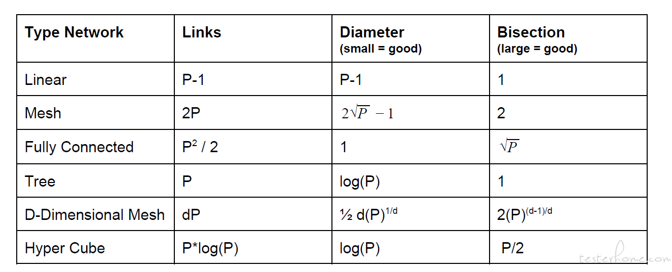
最简单的拓扑网络结构。
Network Types:
1D → Linear
2D → Mesh
Fully Connected = every node has a direct connect to every other node.

网络主要参数：
Links : number of connections (Links).
Diameter: the longest shortest path.
Bisection Width：the minimum number of links that have to be removed to cut the network
into two equal groups of nodes.

其他拓扑结构：
1.tree(FatTree)
2.D-Dimensional Mesh
3.Hyper Cube

Hyper Cube 是一个很神奇的结构

各拓扑结构的性能总结：

Congestion = maximum number of logical edges that map to a physical edge.
Lower Bound on Congestion
Bx → physical bisection width
L → logical edges cut
C>=L/Bx>=BL/ Bx
If you know the congestion. you’ll know how much worse the cost of your algorithm will be on
a physical network with a lower bisection capacity.

L2.4 Distributed Matrix Multiply

Matrix Multiply: Basic Definitions

C ← C + A*B → This is the dot product of row A and column B and accumulating the sum into
the output.
The Matrix Multiply as Parallel pseudo code:

Parfor i ← 1 to m do
  parfor j ← 1 to n do
     let T[1:k] = temp array
     parfor l ← 1 to k do
         T[l] ← A[i,l] . B[l,k]
     C[i,j] ← C[i,j] + reduce(T[:])

W(n) = O(n 3 )
D(n) = O(log n)

** According to Loomis and Witney: The volume of I is ….. |I| <= √|sA| |sB| |sC|**

1D Algorithms

Using Block Row Distribution : this means each node gets n/P rows. (assume the matrices are
square and that n is divisible by P).
计算结构如下图所示：

Block Row Distribution Pseudo Code

let A’[1: n/P] [1:n] = local part of A,B’, C’ = same for B, C
let B’’[1:n/P][1:n] = temp storage
let r next ← (RANK + 1) mod P
let r prev ← (RANK + P-1) mod P
for L ← 0 to P-1 do
   C’[:][:] += A’[:][...L…] . B’[...L…][:] (...L… is a placeholder for the local indices)
   sendAsync (B’ → r next ) (send the local buffer to the next processor)
   recvAsync (B’’ ← r prev ) (receive from the previous processor) 
   wait(*) (wait for send and recv to complete)
   swap(B’, B’’) (swap the receive buffer with the compute buffer)

1D Algorithm Cost

The cost of the algorithm is …
τ = time per "flop" (flop means …1 floating point multiply or add)
Total time is …. Tc omp( n,P) = 2τ n3 / P
How much time is spent on communication?
B’ is the only data communicated. It’s size is n/P words by n columns so n2/P words.
There are P sends that have to be paid for.
So the total cost of communication is : αP + βn2

sendAsync (B’ → r next )
recvAsync (B’’ ← r prev )
C’[:][:] += A’[:][...L…] . B’[...L…][:]

上面的代码稍微替换一下，可以得到：
Recall the running time: T1D, overlap(n;P) = max(2τn3/P, αP + βn2)

Efficiency and the 1D Algorithm

Recall the running time: T1D, overlap(n;P) = max(2τn3/P, αP + βn2)
Speedup: S1D(n;P) ≡ T*(n) / T1D(n;P) = P / max(1, 1/2 * α/τ * P2/n3 + 1/2 * β/τ * P/n )
= θ(P)
Parallel Efficiency = Speedup / P = E(n; P)
A parallel system is efficient if its parallel efficiency is constant. This occurs when: n = Ω(P)
Isoefficiency Function is: n = Ω(P) → the value of P that n must satisfy to have constant parallel efficiency.

reduce Isoefficiency

E(n;P) = S(n;P)/P = T * (n) / P*T(n;P)
Parallel Cost = P*T(n;P) = 1/((1 + P/τ) log P + (α/τ) ( log P)/n
τ = time per scalar add
Ttree(n;P) = τnlog P + αlog P + βnlog P

A 2D Algorithm SUMMA

算法结构如下：

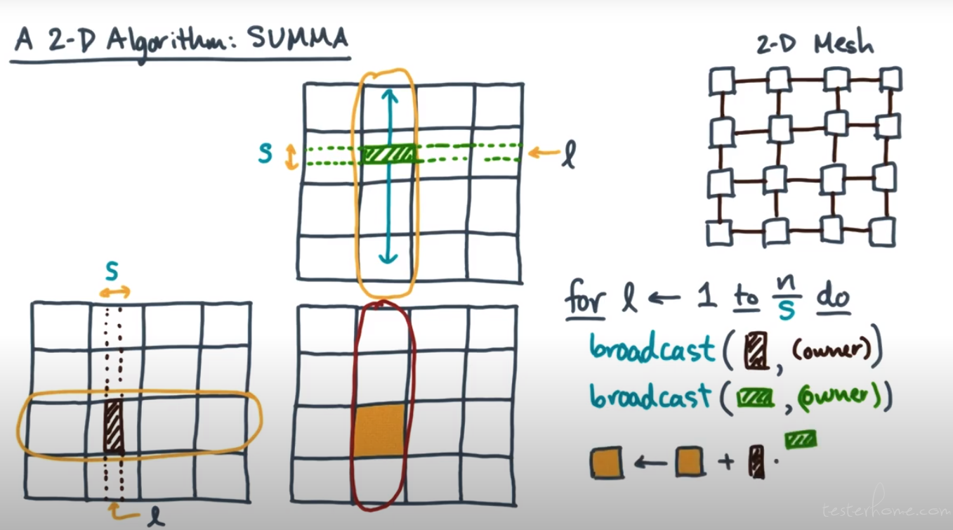
Assume: nxn matrices, √P √P mesh, √Pand s both divisible by n.
TSUMMA(n;P, s) = n/s * (2τ * (n2s/P) + Tnet(n;P, s)
= 2τn3/P + Tnet(n;P, s)

SUMMA Communication Time

Tnet = O(α * n/s * log P + β * n2/√P * log P) → Tree
Tnet = O(α * n/s * P + β * n2/√P) → Bucket

Efficiency of 2D SUMMA

主要看 ntree

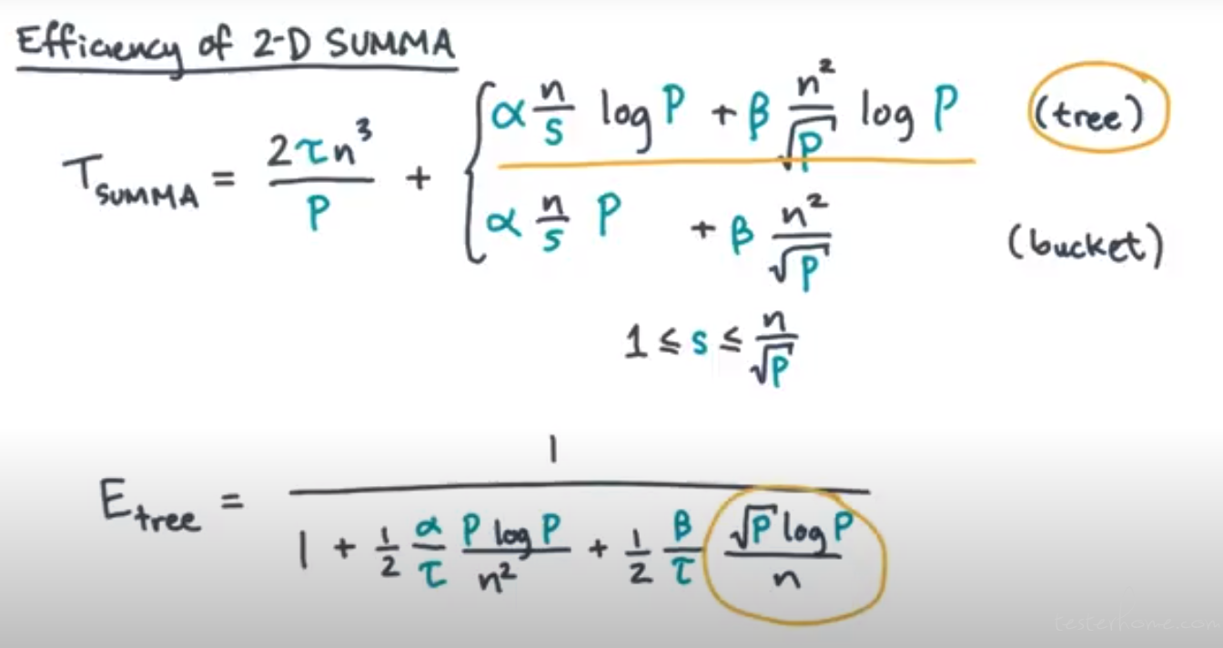
** ntree(P) = Ω(√P log P)**
n1D(P) = Ω(P)
nbucket(P) = Ω(P5/6)
The bucket is slightly worse than the tree, it trades a higher latency cost for a lower
communication cost.

SUMMA Memory

The amount of memory needed for SUMMA is:
MSUMMA = 3 * n2/P + 2 * s * n/√P)

A Lower Bound on Communication

SA, SB, Sc→ the set of unique elements of each matrix seen in this phase.
Max # multiplies per phase ≤ √(|SA| * |SB| * |SC| )≤ 2 * √2 * M3/2

推导过程

words communicated by 1 node ≥ (# full phases) * M

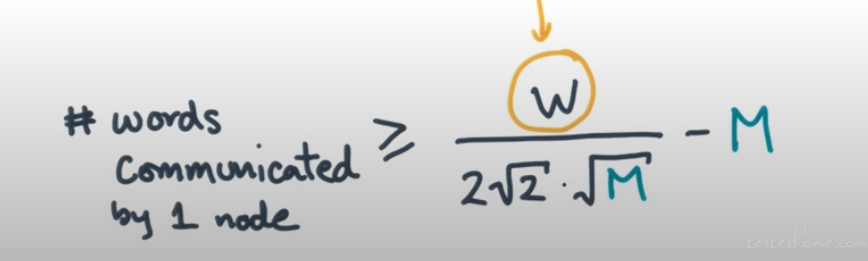
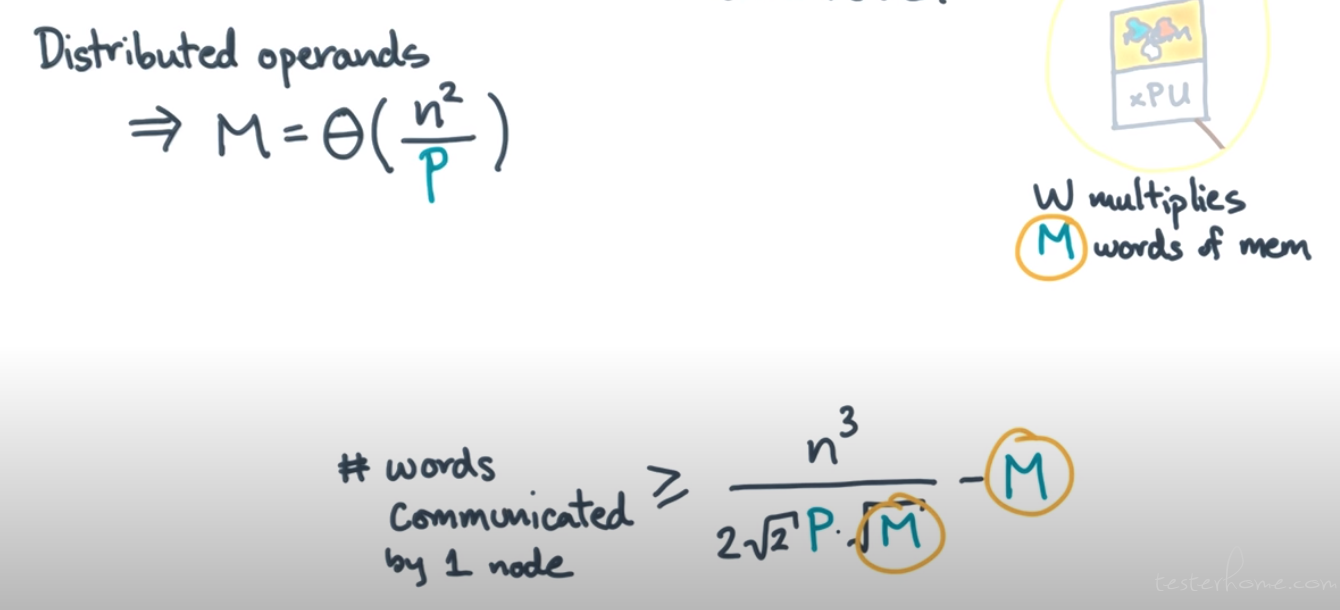
最大消息长度就是 M。

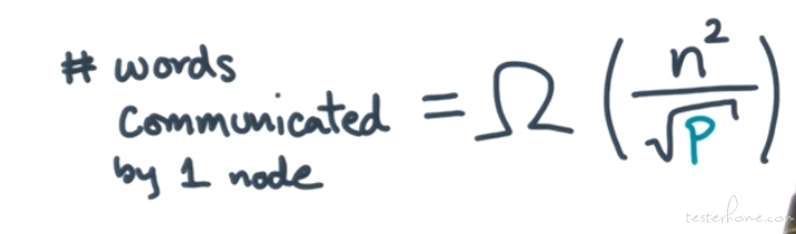
Tnet(n;P) = Ω(α * √P + β * n2/√P)

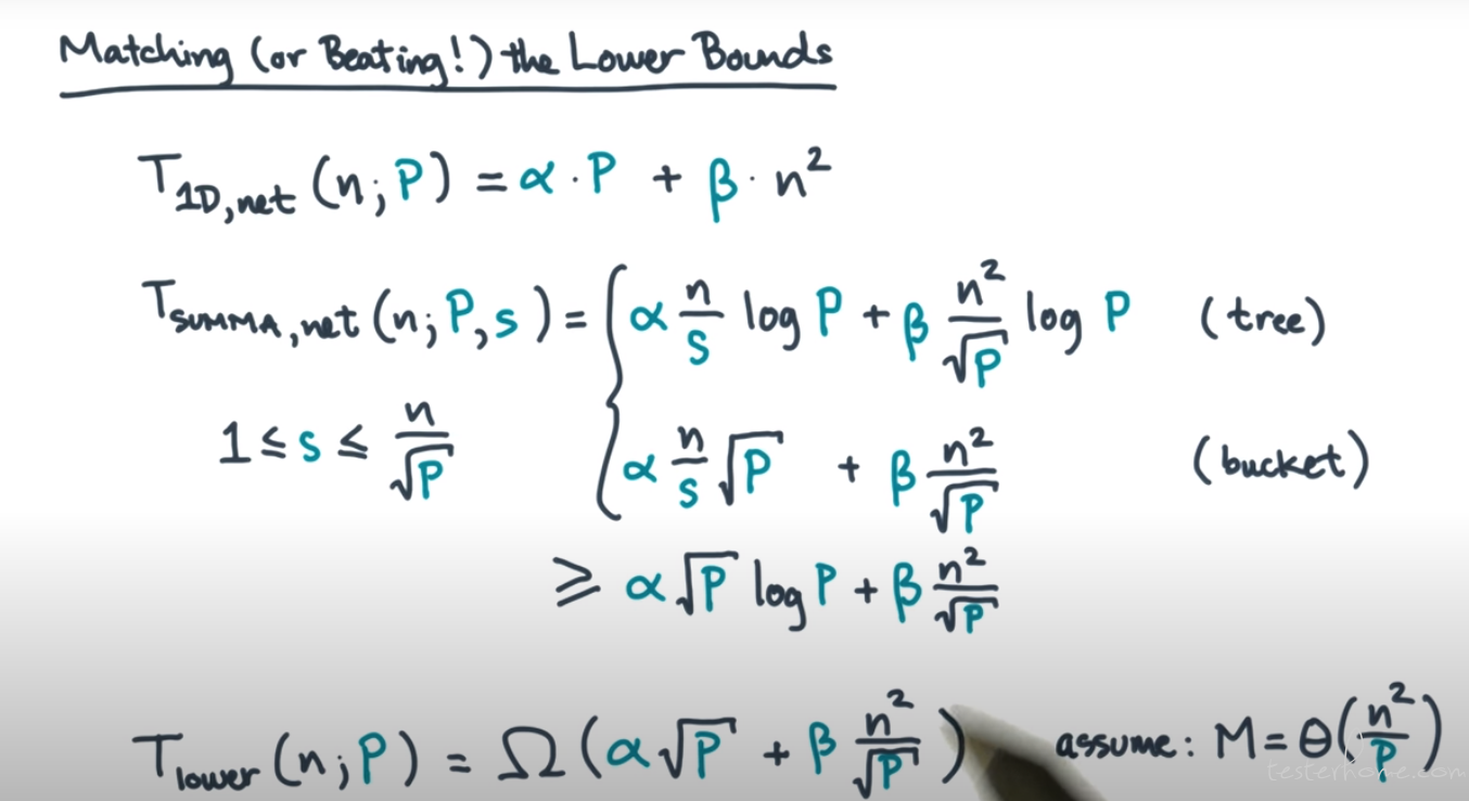
TL ower( n;P) = Ω( α√P + β * n/√P ) assume: M=θ(n 2/P)
从 Cannon 算法而来。